Schnider et al. 1998 - Propofol Pharmacokinetics
Glossary
- plasma, or the bloodstream. This is where propofol is directly infused. It is denoted either $x_1$ when describing absolute drug amount (i.e. $\text{mg}$ or $\mu\text{g}$) or $C_1$ when describing drug concentration (i.e. $\frac{\mu \text{g}}{\text{mL}}$).
- rapidly equilibrating tissue ($x_2$ or $C_2$). This compartment represents tissues that have a high blood supply relative to their size.
- slowly equilibrating tissue ($x_3$ or $C_3$). This compartment represents tissues with poor perfusion, such as adipose tissue (fat).
Paragraph-by-Paragraph Commentary, but Why?
This writeup is part of an ongoing effort to go through the foundational anesthesia literature in excruciating detail, paragraph by paragraph, to ensure that every concept behind the FluxSim Simulator Library is fully understood (by me, the developer). Each section of the paper is followed by commentary and notes that provide the necessary context for full understanding.
Three-compartment PK model. Propofol enters the plasma compartment and distributes to rapid and slow peripheral compartments via Cl₂ and Cl₃. Metabolic clearance Cl₁ eliminates drug from plasma.
Abstract - Background
This paper concerned propofol, a fast-acting intravenous medication used to induce and maintain general anesthesia. It specifically aimed to investigate
- the influences of administration (bolus vs. infusion)
- if the pharmacokinetics of propofol are linear with dose
- the effect of patient covariates on propofol pharmacokinetics
- EDTA on the pharmacokinetics of propofol
Commentary and Notes
Abstract - Methods
Twenty-four healthy volunteers aged 26 to 81 years old were administered the following:
- A bolus dose of propofol
- 1 hour later, a randomly assigned infusion rate $u_p$ for 60 minutes. $$u_p \in \{25, 50, 100, 200\} \ \left[ \mu \text{g} / \text{kg} / \text{min} \right] $$
Each volunteer was studied twice -- once with propofol containing EDTA and once without propofol containing EDTA. The influence of the method of administration and of the patient covariates was explored by fitting a three-compartment mamillary model to the data. The influence of EDTA was investigated by direct comparison of the measured concentrations in both sessions.
Commentary and Notes
I'm thankful for volunteers.
Abstract - Results and Conclusions
- The concentration of propofol ($C_e$) administered with and without the preservative EDTA were not significantly different.
- The concentration measurements of propofol after the bolus doses were significantly underpredicted by the parameters obtained from the infusion data.
- The kinetics of propofol were linear within the range $ [25, 200] \ \frac{\mu\text{g}}{\text{kg} \cdot \text{min}} $ inclusively.
- Age was a significant covariate for the volume and clearance of the rapid equilibriating compartment $x_2$.
- Weight, height, and lean body mass were significant covariates for the metabolic clearance of propofol.
Commentary and Notes
It is interesting that the concentration of propofol after the bolus doses was much higher than predicted by the three-compartment model. I think this suggests that there is some sort of bound to the model, and going beyond that bound will result in inaccuracies to the predictions (an extrapolation issue). To account for this we could investigate adding non-linearities on the flux of propofol out of plasma into the other compartments.
Introduction
Commentary and Notes
We will now do a deep dive by going through the full paper paragraph by paragraph For each paragraph, I will provide notes and commentary that provides the necessary context for full understanding.
Introduction [Paragraph 1]
"THE pharmacokinetics of propofol have been widely studied and reported. [1-7] An unresolved issue in these reports is whether the pharmacokinetics of propofol change with dose and method of administration. The clearance of drugs with hepatic extraction ratios approaching 1 is limited by blood flow in the liver. For drugs with flow-dependent clearance, such as propofol, changes in blood flow in the liver cause proportional changes in clearance. Most anesthetic agents, including propofol, reduce blood flow in the liver. It is probable, a priori, that propofol changes its own clearance. This has been found in dogs [8] but has not been reported in humans, although there have been some suggestive studies. [9]"
This sets the stage for why they tested boluses vs. infusion. They will ultimately show that administering large boluses results in non-linear pharmacokinetics that are not captured by the linear three-compartment model. However, they will end up showing that propofol clearance IS linear within the reasonable infusion rate ranges $u_p \in [25, 200] \ \frac{\mu\text{g}}{\text{kg} \cdot \text{min}}$.
What is "hepatic extraction ratio"? It is the efficiency with which the liver metabolizes a drug, quantified as a fraction of the drug removed from the blood during its passage through the liver.[2] A high hepatic extraction ratio (close to 1) means that blood flow itself will be the bottleneck of clearance, not the metabolic ability of the liver.
Bloodflow was found to be a function of age (as we will say later in the paper). Therefore, clearance rate was found to be a function of age. We will see that the clearance of liver is linear in the three-compartment model: $$ Cl_1 = \sigma_5 + \sigma_{11} \cdot (\text{Age} - 53) $$ Note that clearance in a PK model means that the it is linearly proportional to the amount in the system. $$ \frac{dx}{dt} = -k \cdot x(t) $$ Linear clearance DOES NOT mean constant clearance. It only means $k$ is constant.
With all of that being said, this paragraph suggests that clearance rate slows down in proportion to drug amount: $$ \frac{dx}{dt} = -\hat{k}(x(t)) \cdot x(t) $$ where $\hat{k}(x(t))$ is a function of $x(t)$, thus making the system non-linear.
Thankfully, this non-linearity exists OUTSIDE of reasonable infusion rates that an anesthesia pump would be infusing. Therefore, the linear model is an acceptable approximation within the reasonable infusion rates.
Introduction [Paragraph 2]
"The influence of age on propofol pharmacokinetics remains unresolved. Several studies, including prior work from our laboratory, [2,10] have suggested that the pharmacokinetics of propofol are age-dependent. Other investigators have not found an effect of age. [1,4,5,7]One possible explanation for the differences in results in prior studies might be the influence of dose, the effect of age possibly being limited to higher or lower doses of propofol."
Commentary and Notes
This paper will support that age is a significant covariate of propofol pharmacokinetics.
Introduction [Paragraph 3]
"Between June 1990 and February 1993, the Centers for Disease Control and Prevention conducted investigations at seven hospitals because of unusual outbreaks of bloodstream infections, surgical site infections, and acute febrile episodes after surgical procedures. Only exposure to Diprivan ® (propofol in a lipid emulsion) was significantly associated with the postoperative complications at all investigated hospitals. [11] The lipid vehicle of Diprivan supports rapid bacterial growth at room temperature. [12-15] To reduce the rate of infection, Zeneca Pharmaceuticals Group (Wilmington, DE), the manufacturer of propofol, issued new guidelines for aseptic handling of propofol. These guidelines reduced but did not eliminate the incidence of infection related to propofol emulsion. Zeneca found that the addition of disodium edetate (EDTA) to the formulation of propofol emulsion significantly reduced the extent to which bacterial growth was supported. Zeneca has received no reports of infection or fever related to administration of propofol in the United States since the release of a new propofol formulation with EDTA in July 1996. The influence of EDTA on the pharmacokinetics of propofol has not been reported, and the Food and Drug Administration required this investigation before release of the new formulation of propofol."
Commentary and Notes
As mentioned previously, propofol's lipid emulsion provides a prime environment for bacterial growth. Therefore, an antimicrobial agent is added to inhibit bacterial proliferation in the event of accidental contamination. EDTA is used in Diprivan (the brand name for propofol), while sodium metabisulfite or benzyl alcohol is used in generic formulations.
Introduction [Paragraph 4]
"The purpose of this study was to (1) examine the influence of method of administration (bolus vs. infusion) and dose (infusion rate) on the pharmacokinetics of propofol; (2) examine the influence of age, height, weight, and gender on the pharmacokinetics of propofol using a population approach; and (3) study the influence of EDTA on the pharmacokinetics of propofol. The null hypotheses were that EDTA, method of administration, dose, age, height, weight, gender, and EDTA do not influence the pharmacokinetics of propofol."
Commentary and Notes
A null hypothesis $H_0$ proposes that there's no effect or differences between certain variables.
Methods
Study Design
"After the study was approved by the Institutional Review Board and after giving written informed consent, 25 American Society of Anesthesiologists status I and II volunteers were enrolled in this study. One volunteer dropped out of the study before completion because of depression and was not included in the analysis. The study design was a randomized, double-blind, age-stratified, two-period, crossover trial. The volunteers were stratified into three age groups -- 18-34 yr, 35-65 yr, and > 65 yr -- of eight volunteers each. Each volunteer was studied twice, receiving (in a randomized, double-blind, crossover fashion) either propofol without EDTA (the commercially available formulation of Diprivan before July 1996) or propofol with EDTA (the commercially available formulation of Diprivan in the United States after July 1996) in each study session. All volunteers received an initial bolus dose over ≈ 20 s of either 2.0 mg/kg for volunteers aged ≤ to 65 yr or 1.0 mg/kg for volunteers aged > 65 yr, followed 1 h later by an infusion administered over 60 min. The infusion rate was assigned according to a nonblinded, randomized design to 25, 50, 100, or 200 $\mu\text{g} \cdot \text{kg}^{-1}\cdot \text{min}^{-1}$, with two volunteers in each age group assigned to each infusion rate."
Commentary and Notes
Let's compare the order of magnitude of the bolus doses with that of the
infusion rates.
For patients $\leq$ 65 years old:
$$u_{bolus_{nom}} = \frac{2}{20} \left[\frac{\text{mg}/\text{kg}}{\text{s}}\right]
\cdot \frac{60}{1} \left[ \frac{\text{s}}{\text{min}} \right]
\cdot \frac{1000}{1} \left[ \frac{\mu \text{g}}{\text{mg}} \right] =
6000 \left[ \frac{\mu\text{g}/\text{kg}}{min} \right]$$
For patients > 65 years old:
$$u_{bolus_{sen}} = \frac{1}{20}
\left[\frac{\text{mg}/\text{kg}}{\text{s}}\right] \cdot \frac{60}{1}
\left[ \frac{\text{s}}{\text{min}} \right] \cdot \frac{1000}{1} \left[
\frac{\mu \text{g}}{\text{mg}} \right] = 3000 \left[
\frac{\mu\text{g}/\text{kg}}{min} \right]$$
Considering minimum and maximum infusion rates from the study:
$$u_{r_{min}} = 25 \left[ \frac{\mu\text{g}/\text{kg}}{min} \right]$$
$$u_{r_{max}} = 200 \left[ \frac{\mu\text{g}/\text{kg}}{min} \right]$$
We can show the order of magnitude difference between the bolus doses
and the infusion rates.
$$ \frac{u_{bolus_{nom}}}{u_{r_{min}}} = 240 \
\left[\vphantom{\frac{a}{b}}\cdot\right] \quad
\frac{u_{bolus_{nom}}}{u_{r_{max}}} = 30 \
\left[\vphantom{\frac{a}{b}}\cdot\right]$$
$$ \frac{u_{bolus_{sen}}}{u_{r_{min}}} = 120 \
\left[\vphantom{\frac{a}{b}}\cdot\right] \quad
\frac{u_{bolus_{sen}}}{u_{r_{max}}} = 15 \
\left[\vphantom{\frac{a}{b}}\cdot\right]$$
Or put simply, the bolus amount is between 30 and 240 times the infusion
rate for those with age less than or equal to 65, and 15 to 120 times
the infusion rate for those with age greater than 65.
This is pertinent when we go to our modeling, as infusion rates $\geq$
200 $\frac{\mu\text{g}/\text{kg}}{\text{min}}$ may be in the non-linear
region, where our linear ODE breaks down.
Practically, if we consider the patient with the maximum weight weight
within the study of 123 kg, we are looking at maximum infusion rate
(still within the linear region) of $u_{max} = 123 \cdot 200 =
24.6 \frac{\text{mg}}{\text{min}}$. Without introducing non-linearities
to the simulation model, we can still limit delivery from the controller
to ensure it does not violate the boundary which would result in
non-linear dynamics (PID controller delivery must be $\leq 200 \
\frac{\mu\text{g}/\text{kg}}{min}$)
Acquisition, Handling, and Processing of Samples
"Propofol was administered via an 18-gauge catheter inserted into a forearm vein. A 20-gauge catheter was inserted into the radial artery for blood pressure monitoring and for sample collection. Samples of 4-7 ml of arterial blood were taken at 0, 1, 2, 4, 8, 16, 30, 60, 62, 64, 68, 76, 90, 120, 122, 124, 128, 136, 150, 180, 240, 300, and 600 min and placed in heparinized tubes. The samples were placed on ice and centrifuged within 2 h of collection. The plasma was transferred to polypropylene tubes and frozen immediately. The tubes were stored at $-20^\circ$ until assayed."
Commentary and Notes
Notice the samples start small $0, 1, 2, 4, 8$ and increase until 60. This is to capture the dynamics of the bolus. Then, at 60, when the infusion portion of the experiment begins, the sampling frequency increases again: $60, 62, 64, 68, ...$
Propofol Assay
"Propofol was assayed using liquid-liquid extraction followed by reverse-phase high-performance liquid chromatography with fluorescence detection. The lower limit of detection was 2.0 ng/ml."
Commentary and Notes
I trust the researchers on the details of their extraction method. Practically, this is describing how they measured propofol concentration in the blood samples.
Pharmacokinetic Analysis [Paragraph 1]
"Influence of Method of Administration. The design of this study was chosen to provide safety and efficacy data about two common types of propofol use, bolus administration and continuous infusion. (The safety and efficacy data are not addressed in this article.) This design also permitted an evaluation of the influence of method of administration on the pharmacokinetics of propofol. The infusion was started 1 h after the bolus dose to (1) permit an adequate period of observation after delivery of the bolus dose, and (2) allow the concentrations of propofol in plasma to decline to low levels before starting the continuous infusion."
Commentary and Notes
So this is a preview that propofol mostly clears from the system within an hour after administration.
Pharmacokinetic Analysis [Paragraph 2]
"For each volunteer, we estimated the individual pharmacokinetics based on the observed concentrations starting 62 min after the bolus dose (2 min after the start of the infusion) using NONMEM.* Although the dose regimen included the bolus dose information, NONMEM did not attempt to fit the model to the observations in the 60 min after administration of the bolus dose. Therefore, the resulting pharmacokinetic parameters described the observations from each individual based on the infusion data only. We then used the infusion-based pharmacokinetics to predict the observations in the 60 min after the bolus injection in the same individual. For this analysis, the two study sessions for each individual were treated as separate studies because the pharmacokinetics during the infusion were compared with the observations immediately after the bolus dose in the same study (i.e., each study served as its own control)."
Commentary and Notes
NONMEM (NONlinear Mixed Effects Modeling) is the gold-standard software tool developed for population pharmacokinetic and pharmacodynamic (PK/PD) analysis. The "Mixed" effects stands for both fixed effects (drug clearances) and random effects (inter-individual variability and residuals).
Here is the summary of their process.
- Fit PK based on blood samples from infusion phase for each patient
- Used those PK parameters to predict the PK of the bolus phase within the same patient
Pharmacokinetic Analysis [Paragraph 3]
"For each of the samples in the first 60 min after the bolus injection, we calculated a ratio of the measured concentration at each time t to that predicted by pharmacokinetics estimated from the infusion data: $$ \text{ratio}(t) = \frac{ \text{Concentration}(t)_{ \text{measured}} } { \text{Concentration}(t)_{\text{predicted}} } $$ If mode of drug delivery has no effect on pharmacokinetics, the ratio in this equation should be 1 (the infusion pharmacokinetics should predict the bolus response). If the ratio differs significantly from 1, then there are statistically (but perhaps not clinically) significant differences in the pharmacokinetics after bolus injection and during continuous infusions."
Commentary and Notes
For each sample $i$, the ratio $R_i$ was calculated as the measured concentration $x_i$ over the predicted PK estimate $\hat{x}_i$. $$ R_i = \frac{x_i}{\hat{x}_i} $$ Remember, the null hypothesis $H_0$ was that the method of administration has no effect, $R_i \approx 1.0$.
Pharmacokinetic Analysis [Paragraph 4]
"We used the infusion data to predict the response to the bolus dose and not the response to predict the infusion data because the response to the bolus dose was observed for only 60 min before the infusion was started. It would not be reasonable to expect the pharmacokinetics estimated from just 60 min of postdose data to predict the observations during the 1-h infusion followed by 8 h of postinfusion data."
Commentary and Notes
I think this is trying to say that it is not reasonable to fit parameters to the one hour of bolus data when they had 9 hours of postinfusion data available.
It also be proved to "not be reasonable" for a second reason -- the bolus data shows non-linearities, while the infusion data can be better approximated with the linear model. This fact was not known until after the study however. But I wouldn't be surprised if they tried both -- fit infusion data and tried to predict bolus, and then fit bolus and tried to fit infusion data.
Pharmacokinetic Analysis [Paragraph 5]
"Influence of Infusion Rate. The four infusion rates selected for this study, 25, 50, 100, and 200 $\mu \text{g} \cdot \text{kg}^{-1} \cdot \text{min}^{-1}$, span the clinical range of infusions of propofol during the maintenance of anesthesia. Had the study started with an infusion, linearity regarding infusion rate could have been determined by dividing all observed concentrations by the infusion rate and demonstrating that the rate-normalized concentrations did not differ between groups. The study design was modestly complicated by the initial bolus dose, whose influence had to be accounted for before dose normalization of the concentrations. This was accomplished by individually fitting a three-compartment model in NONMEM to all the observations in each study session and then calculating the contribution of the bolus dose at each point in time to the observed concentration. The contribution of the bolus dose was subtracted from the observed concentrations during and after the infusion, providing an estimate of the concentration that would have been observed had no bolus dose been administered before the infusion."
Commentary and Notes
I appreciate the honesty here. The boluses have to be accounted for, especially if the propofol has not entirely cleared the system. Luckily, we can time travel 28 years to present day, and I'm sure the models have come a long way. Surely, many experiments have reproduced the finding that propofol pk is largely linear within the clinical range of the maintenance period.
I'm just now diving into anesthesia, and I cannot wait to dig into future research. For now, we will trust that their NONMEM models were reasonably able to subtract propofol concentration from the samples taken from the infusion phase.
Pharmacokinetic Analysis [Paragraph 6]
"The influence of infusion rate was determined by dividing the observed concentrations, less the adjustment for the bolus dose, by the infusion rate. The resulting time versus concentration profiles were then graphed and visually examined for evidence of nonlinearity. In contrast to the more traditional assessment of linearity by comparing area under time concentration curves, this method provides an assessment of linearity that is true to the polyexponential nature of anesthetic pharmacokinetics. We also examined the concentrations at 68, 76, 90, and 120 min using Kruskal-Wallis nonparametric analysis of variance. A probability value $\lt$ 0.05 was considered significant."
Commentary and Notes
So they basically took all samples $x_i \in X$, subtracted the bolus dose adjustment from each sample $x_{\text{adj}_i}$ and divided by the infusion rate $u_r$. $$ x_{\text{normalized}_i} = \frac{x_i - \hat{x}_{\text{adj}_i}}{u_r} $$ If linear, we would see all $x_{\text{normalized}_i}$ overlapping. For example, let's assume propofol PK are linear with dose. Meaning, if we double the infusion rate, we double the concentration. Let's suppose we have two infusion rates $$ u_1 = 100 \left[ \frac{\mu \text{g} / \text{kg}}{min} \right], \quad u_2 = 25 \left[ \frac{\mu \text{g} / \text{kg}}{min} \right] $$ If linear, we would expect that the normalized samples are identical. Let's call propofol concentration in samples from a patient receiving infusion rate one "$x$" and samples from a patient receiving infustion rate two "$y$". $$ \frac{x_i - \hat{x}_{\text{adj}_i}} {u_1} = \frac{y_i - \hat{y}_{\text{adj}_i}} {u_2} \ \forall \ i \in \text{infusion phase} $$ in this case, $ u_1 = 4 \cdot u_2 $, resulting in $$ \frac{x_i - \hat{x}_{\text{adj}_i}} {4 \cdot u_2} = \frac{y_i - \hat{y}_{\text{adj}_i}} {u_2} \implies x_i - \hat{x}_{\text{adj}_i} = 4 \cdot \left( y_i - \hat{y}_{\text{adj}_i} \right) $$ So we expect that once both concentrations are adjusted for residuals from the bolus phase, the concentration of patient 1 is four times that of patient 2, because their infusion rate was 4 times that of patient 2. What is unclear is the effect of age, body weight, and other covariates on this linearity analysis at this point in the study design.
Pharmacokinetic Analysis [Paragraph 7]
"Influence of Subject Covariates. We used the approach described by Mandema et al., [16] implemented as reported by Minto et al. for remifentanil, [17] to develop a population pharmacokinetic model for the new EDTA-containing propofol emulsion, because this is the only propofol formulation now available in the United States. All concentrations from the sessions where propofol with EDTA was given were used in the analysis. Two-and three-compartment population pharmacokinetic models were estimated by NONMEM using the first- order conditional estimation and $\eta - \epsilon$ interaction to reduce the influence of model misspecification. Specifically, the eta-epsilon interaction option accounts for the interaction between intra- and interindividual variability.** The structural model was chosen according to the objective function (minus twice the log likelihood [-2LL]), with a decrease of 6.6 for one additional parameter considered significant $(P \lt 0.01)$."
Commentary and Notes
There is a lot to unpack in this paragraph.
Let's get the simple thing out of the way. Only using propofol with EDTA was a practical decision. That formulation was the only one actually being manufactured in the US at the time, so that is the one that matters clinically.
Now, the more complicated math-heavy portion. The choice between a two- and three-compartment model wasn't made from first principles (at least not explicitly mentioned here). Rather, they tried both and let the data decide. Adding more compartments always improves the fit a little -- more free parameters means more flexibility, which always reduces error, but risks overfitting and makes identifiability harder to prove. So they required the improvement to clear a statistical bar before accepting the more complex model.
To understand the bar, we first need to understand likelihood. Given a model with a fixed set of parameters, the likelihood $L$ is the probability of observing the data you actually measured. For a set of $n$ independent observations $y_i$ with predicted values $\hat{y}_i$ and measurement error $\sigma$, a simple Gaussian likelihood looks like: $$L = \prod_{i=1}^{n} \frac{1}{\sigma\sqrt{2\pi}} \exp\!\left(-\frac{(y_i - \hat{y}_i)^2}{2\sigma^2}\right)$$ Because this product of many small numbers becomes numerically impractical, we take the log: $$\ln(L) = -\frac{n}{2}\ln(2\pi\sigma^2) - \frac{1}{2\sigma^2} \sum_{i=1}^{n}(y_i - \hat{y}_i)^2$$ A higher log likelihood means the model's predictions are closer to the observed data, i.e. a better fit. NONMEM maximizes this over all parameters to find the best fit, and reports $-2\ln(L)$ (so that smaller is better, and the $\chi^2$ comparison works out cleanly).
Back to the statistical test, which is the drop in -2LL between the simpler and more complex model: $$\Lambda = (-2\ln(L_0)) - (-2\ln(L_1))$$ where $L_0$ is the likelihood of the simpler model and $L_1$ is the likelihood of the more complex model. By Wilks' theorem, $\Lambda$ is asymptotically $\chi^2$ distributed (as samples $\rightarrow \infty$), with degrees of freedom equal to the number of added parameters. The factor of 2 isn't arbitrary. It comes from a second-order Taylor expansion of the log likelihood around its maximum, and it's exactly what makes the statistic land on the $\chi^2$ scale without any additional scaling.
For one additional parameter, the $\chi^2$ critical value at $p < 0.01$ is 6.63 — which is where the 6.6 threshold comes from. In plain terms: if adding a compartment drops the -2LL by less than 6.6, there is more than a 1% chance that improvement happened by random chance alone, so the extra complexity is not justified.
The η-ε interaction is a technical correction in NONMEM that accounts for the fact that patients who are outliers (high inter-individual variability) also tend to have larger residual errors. Ignoring that correlation biases the parameter estimates, so they corrected for it.
Pharmacokinetic Analysis [Paragraph 8]
"The interindividual error on each of the model parameters ($V_1$, $V_2$, $V_3$, $\text{Cl}_1$, $\text{Cl}_2$, $\text{Cl}_3$) was modeled using a log-normal variance model: $$ P_i = \theta_{TV} e^{\eta_i} $$ where $P_i$ is the parameter of an individual and $\eta_i$ is a random variable that describes the interindividual variability between the parameter from the value in the typical individual. The residual intraindividual error was modeled with a constant coefficient of variation model. Empirical Bayesian estimates [18,19] of the pharmacokinetic parameters of each individual were calculated. Bayesian statistics applied to pharmacokinetics balance the uncertainty in the measured concentrations against the uncertainty in a person's parameter estimates. The relation between the subject covariates (age, gender, weight, height, lean body mass [LBM], and body surface area [BSA]) and the pharmacokinetic parameters was explored using a generalized additive model (GAM) implemented in S plus. [16,17] The GAM function performed a stepwise search to find the significant covariates and best form (linear or nonlinear) of each important covariate."
Commentary and Notes
The log-normal model $$ P_i = \theta_{TV} e^{\eta_i} $$ is saying: take the typical population value $\theta_{TV}$, then multiply it by a random factor $e^{\eta_i}$ to get the individual patient's value. The exponential is used instead of simple addition because PK parameters like clearance and volume can never be negative, and the exponential guarantees that. It also makes variability multiplicative -- a patient who is 30% above typical stays 30% above regardless of what the typical value is.
The "log-normal" name might be confusing since the equation just looks like an exponential. The name comes from taking the log of both sides: $$ \ln (P_i) = \ln (\theta_{TV}) + \eta_i $$ Since $\eta_i$ is normally distributed, $\ln(P_i)$ is normally distributed. This means $P_i$ itself follows a log-normal distribution across the population. In short, the equation is exponential. The distribution of $P_i$ is log-normal.
The constant coefficient of variation error model just means measurement noise scales with the predicted concentration. If you're predicting a high concentration, the absolute error is larger, but the relative error stays the same. This is more realistic than assuming a fixed absolute error across all concentration levels.
Empirical Bayes is a practical compromise between two bad extremes. Fitting each patient independently gives noisy estimates when you only have a few blood draws per patient. Using only the population mean ignores the individual's own data entirely. Empirical Bayes balances both. It pulls each patient's estimate toward the population mean, with the strength of that pull depending on how sparse their data is. More data = less pull.
The GAM covariate search is essentially automated model selection for the covariate relationships. Instead of assuming upfront that age has a linear effect on clearance, GAM tests each covariate, finds which ones significantly improve the fit, and figures out whether the relationship is linear or nonlinear. So the final covariate model was discovered from the data rather than assumed from physiology.
The two-step pipeline is worth making explicit: NONMEM first returned one set of individual PK parameters {$V_1$, $V_2$, $V_3$, $\text{Cl}_1$, $\text{Cl}_2$, $\text{Cl}_3$} per patient for a total of 24 sets. Separately, they had each patient's demographics {age, weight, height, sex, LBM, BSA}. They then handed both tables to S-Plus and let GAM find which demographics correlated with which PK parameters.
S-Plus was a commercial statistical programming language widely used in the 1990s, and was essentially the predecessor to R. It has nothing to do with NONMEM. If this paper were written today, the GAM step would almost certainly be done in R, which was created as a free open-source reimplementation of S-Plus and has since replaced it entirely.
Pharmacokinetic Analysis [Paragraph 9]
"Lean body mass was calculated from gender, weight (in kilograms), and height (in centimeters): men, LBM = 1.1 x weight - 128 x (weight/height)${}^2$; women, LBM = 1.07 x weight - 148 x (weight/height)${}^2$. Body surface area was calculated from weight (in kilograms) and height (in centimeters) [20]: BSA = weight${}^{0.425}$ $\pm$ height${}^{0.725}$ x 0.007184."
Commentary and Notes
We have reached our first calculations that are part of the FluxSim Simulator Library! $$\begin{aligned} \text{LBM}_{\text{M}}(\text{wt}, \text{ht}) &= 1.10 \cdot \text{wt} - 128 \cdot \left(\frac{wt}{ht}\right)^2 && \left[ \text{kg} \right] \\ \text{LBM}_{\text{F}}(\text{wt}, \text{ht}) &= 1.07 \cdot \text{wt} - 148 \cdot \left(\frac{wt}{ht}\right)^2 && \left[ \text{kg} \right] \\ \end{aligned}$$ and $$\begin{aligned} \text{BSA}(\text{wt}, \text{ht}) &= \text{wt}^{0.425} \cdot \text{ht}^{0.725} \cdot 0.007184 && \left[ \text{m}^2 \right] \end{aligned}$$ Note that the $\pm$ in the original paper for $\text{BSA}(\text{wt}, \text{ht})$ was a typo. I double checked with the reference.
Pharmacokinetic Analysis [Paragraph 10]
"The covariates identified by the GAM analysis were then incorporated into the structural model and tested with NONMEM for their statistical significance, using the NONMEM objective function and the standard errors of the estimated parameters. A parameter was deleted from the final model if $\pm$ 2 x SE of the parameter included 0."
Commentary and Notes
Table 2 from the paper reports 11 parameter estimates, $\{ \theta_1, \theta_2, ..., \theta_{11} \}$ and their standard errors (SE). For each of these parameters, if NONMEM found that zero was within $\pm 2 \cdot \text{SE}$, then the variable was thrown away. This means, that there was $\ge \approx 5\%$ that the variable had no effect.
Pharmacokinetic Analysis [Paragraph 11]
"As used previously, [21] we described the quality of the goodness of fit using the weighted residual (WR), defined as (Measured - Predicted)/Predicted."
Commentary and Notes
WR is preferred over something like RMSE, because propofol concentration spans several orders of magnitude over the range of the study, and RMSE at higher concentrations would drown out RMSE at lower concentrations, when both should be treated equally with a percentage-based metric.
Pharmacokinetic Analysis [Paragraph 12]
"The median weighted residual (MDWR), calculated as the median WR over all of the observations, is a measure of bias. The median absolute weighted residual (MDAWR), calculated as the median of the absolute value of the WR, is a measure of inaccuracy of the fit. We visually examined the goodness of fit by plotting the measured/predicted values on a logarithmic scale for each volunteer as a function of time. The WRs were only calculated for observations from the new EDTA formulation, as these were the data used to estimate the pharmacokinetic model."
Commentary and Notes
MDWR is a measure of bias. If MDWR is positive, measured is systematically higher than predicted, meaning the model is underpredicting. If MDWR is negative, the opposite is true. The median is more robust to outliers (as compared to mean).
MDAWR is a measure of inaccuracy. It strips away the sign so that positive and negative error can't cancel out and mask a bad model. Thus, it tells you if the model is wrong on average.
Pharmacokinetic Analysis [Paragraph 13]
"We also calculated the ability of the model to describe the concentrations observed after administration of propofol emulsion without EDTA. Because these data were not used to estimate the model parameters, the ability of the model to describe these observations represents a measure of the performance of this model. It also helps measure the influence of EDTA on the pharmacokinetics of propofol. These measures were therefore based on the performance error (PE), also defined as (Measured - Predicted)/Predicted."
Commentary and Notes
The performance error formula is identical to the weighted residual formula $$ P_{e_i} = \frac{ \text{Measured}_i - \text{Predicted}_i }{ \text{Predicted}_i } $$ The difference is only the data it applies to. WR was calculated on the EDTA data (measured goodness of fit), and PE was calculated on the non-EDTA data (measures out-of-sample performance). If $\text{PE}_{ \text{non-EDTA} } \approx \text{WR}_{ \text{EDTA} }$, it implies that EDTA doesn't meaningfully change the pharmacokinetics of propofol.
Pharmacokinetic Analysis [Paragraph 14]
"We calculated the MDPE and MDAPE as described for the WR, mutatis mutandis."
Commentary and Notes
"Mutatis mutandis" is Latin for "with the necessary changes made". Here, it just means they calculated median PE and median absolute PE just like they did for WR.
Pharmacokinetic Analysis [Paragraph 15]
"Because age did prove to be a significant covariate (see results), we performed an additional analysis to ensure that this finding was not due simply to the lower bolus dose given to the elderly volunteers. As in the section on the influence of infusion rate, the concentrations that were corrected to remove the contribution of the bolus dose and normalized to dose (normalized, corrected concentrations) were compared with age, and a linear least-squares fit was done for four representative time points (68, 76, 128, and 136 min). Then the full covariate model was used to predict the concentration after a 60-min infusion at 200 $ \left[ \mu \text{g} \cdot \text{kg}^{-1} \cdot \text{min}^ {-1} \right] $ into a typical volunteer (77 $\left[ \text{kg} \right]$, 175 $ \left[ \text{cm} \right] $, female) at ages 25, 50, and 75 yr, and those predicted concentrations were normalized. The predictions of the model were compared with the normalized, corrected concentrations from the volunteers."
Commentary and Notes
Recall from the study design, that patients over 65 years old received half the normalized bolus dose, $1 \left[ \frac{ \text{mg} } { \text{kg} } \right]$ rather than $2 \left[ \frac{ \text{ mg }} { \text{kg} } \right] $. So Schnider et. al are doing their due diligence here, ensuring that the effects of age on the fitted parameters was not due to the difference in bolusing regime.
Pharmacokinetic Analysis [Paragraph 16]
"Influence of Disodium Edetate on Pharmacokinetics of Propofol. Each volunteer received virtually identical bolus doses of propofol and infusions in each of the two sessions, permitting direct comparison of concentrations of propofol in plasma between the two sessions. For each individual we calculated the ratio at each time $t$ of the concentrations measured when propofol without EDTA was administered with the concentrations measured when propofol with EDTA was administered: $$ \text{ratio}(t) = \frac{ \text{Concentration}(t)_{ \text{without EDTA} } }{ \text{Concentration}(t)_{ \text{with EDTA} } } $$ We plotted this ratio over time for all individuals to examine any systematic deviations from 1. We also calculated confidence bounds about each point for a probability of 0.95. A Bonferroni correction was not performed to maintain sensitivity to any deviation of the ratio from 1."
Commentary and Notes
At each time point $t$, the ratio is computed once per volunteer, giving 24 ratio values. The 95% confidence interval on the mean ratio is: $$\text{CI}_{95\%} = \mu_i \pm 2.07 \cdot \frac{\sigma_i}{\sqrt{n}}$$ where $\mu_i$ is the mean ratio across all volunteers for sample {i}, $\sigma_i$ is the standard deviation of those ratios, $n$ is the number of samples (24 patients = 24 samples per $t$) and $2.07$ is the t critical value for 23 degrees of freedom representing the 95% confidence bounds. This interval tells you where the true mean ratio is likely to fall. If it contains 1, there is no statistically significant difference between the two formulations at that time point.
Since this test is repeated at every sample time, applying the Bonferroni correction would widen the CI at each time point, making it easier for 1 to stay inside. $$ \text{CI}_{95\% Bonferroni } = \mu_i \pm 3.69 \cdot \frac{ \sigma_i }{ \sqrt{n} } $$ By skipping it, they kept the CI narrower, making it harder to confirm no effect. The fact that 1 still fell inside the bounds at every time point strengthens their "no effect" conclusion.
Results [Paragraph 1]
"The demographic data of the study population are summarized in table 1 by order of infusion group and age group. The ages were divided evenly between the different doses by study design. The study was not formally stratified by gender. By chance, only one woman was included in the 25-$\mu \text{g} \cdot \text{kg}^{-1} \cdot \text{min}^{-1}$ infusion group, and only one man was included in the 200-$\mu \text{g} \cdot \text{kg}^{-1} \cdot \text{min}^{-1}$ infusion group. Taking the two low-dose and the two high-dose groups together, only three women were included in the 25- and 50-$\mu \text{g} \cdot \text{kg}^{-1} \cdot \text{min}^{-1}$ infusion group, but eight women were assigned randomly to the 100- and 200-$\mu \text{g} \cdot \text{kg}^{-1} \cdot \text{min}^{-1}$ group. These differences were not statistically significant (Pearson's chi-square test with Yates's continuity correction). The groups were otherwise homogeneous regarding the observed covariates."
Commentary and Notes
| Inf | Age (yr) | Weight (kg) | Height (cm) | Gender |
|---|---|---|---|---|
| 25 | 34 | 46.3 | 158 | F |
| 25 | 31 | 123 | 196 | M |
| 25 | 62 | 79.4 | 170 | M |
| 25 | 65 | 79.4 | 182 | M |
| 25 | 77 | 74.8 | 183 | M |
| 25 | 70 | 62.6 | 175 | M |
| 50 | 30 | 64.4 | 170 | M |
| 50 | 27 | 74.8 | 188 | M |
| 50 | 46 | 93.4 | 182 | M |
| 50 | 41 | 90.7 | 178 | F |
| 50 | 72 | 88.4 | 183 | M |
| 50 | 75 | 64.4 | 168 | F |
| 100 | 29 | 95.2 | 188 | M |
| 100 | 26 | 88.4 | 178 | M |
| 100 | 55 | 44.7 | 168 | F |
| 100 | 51 | 79.8 | 175 | F |
| 100 | 81 | 74.8 | 178 | M |
| 100 | 72 | 70.3 | 170 | F |
| 200 | 31 | 91.2 | 180 | F |
| 200 | 25 | 63.5 | 158 | F |
| 200 | 62 | 86.2 | 180 | M |
| 200 | 38 | 88.4 | 173 | F |
| 200 | 74 | 70.3 | 160 | F |
| 200 | 75 | 44.4 | 155 | F |
The gender imbalance across dose groups was tested using Pearson's chi-squared with Yates's continuity correction. Yates's correction is only applicable to a 2x2 contingency table, so the four dose groups were likely collapsed into two: low dose (25 and 50 µg/kg/min) and high dose (100 and 200 µg/kg/min). The table then has 2 rows (M/F) x 2 columns (low/high), giving 1 degree of freedom.
| Male | Female | |
|---|---|---|
| Low Dose | 9 | 3 |
| High Dose | 4 | 8 |
The null hypothesis is that gender assignment is independent of dose group -- essentially a fair coin flip. The test statistic without Yate's correction is: $$ \begin{aligned} \chi^2 &= \sum \frac{(O - E)^2}{E} \\ \chi^2 &= \frac{(9-6)^2}{6} + \frac{(3-6)^2}{6} + \frac{(4-6)^2}{6} + \frac{(8-6)^2}{6} \\ \chi^2 &= \frac{9}{6} + \frac{9}{6} + \frac{4}{6} + \frac{4}{6} \\ \chi^2 & \approx 4.33 \end{aligned} $$ 4.33 is above the critical value of 3.84 at p = 0.05, so without Yate's correction, the imbalance would be borderline significant. With Yate's correction, it drops below the threshold. $$ \begin{aligned} \chi^2_{\text{Yates}} &= \sum \frac{(|O - E| - 0.5)^2}{E} \\ \chi^2_{\text{Yates}} &= \frac{2.5^2}{6} + \frac{2.5^2}{6} + \frac{1.5^2}{6} + \frac{1.5^2}{6} \\ \chi^2_{\text{Yates}} &\approx 2.83 \end{aligned} $$ where $O$ is the observed count and $E$ is the expected count in each cell. The 0.5 correction makes the test more conservative, appropriate for small samples. The result was not significant, confirming the gender imbalance was consistent with random assignment.
Results [Paragraph 2]
"All measured concentrations were included in the pharmacokinetic analysis. In each of two volunteers, one measurement for concentration in plasma was not available because the tube broke during centrifugation. Therefore, for 46 study sessions, we had 22 measurements of concentration in plasma, and for 2 study sessions we had 21 measurements. No points were lower than the limit of quantification of the assay. The investigators could not clinically distinguish a difference between the volunteers who received EDTA and those who did not."
Commentary and Notes
Probably an intern...
Results - Influence of Method of Administration [Paragraph 3]
"Figure 1 (top) shows the ratio of concentrations after bolus injection to the concentrations predicted from the infusion data. The bias is statistically significant (Figure 1, middle), as shown by the mean and 95% confidence interval for the ratio of measured to predicted value. The 2- and 4-min samples show a statistically significant negative bias. At all other times the bias is positive and statistically significant. Figure 1(bottom) shows that, although the bias may be statistically significant, it pales in comparison to the overall interindividual variability in concentration after bolus injection. The predictions of the pharmacokinetic models based on the infusion data alone (Figure 1, dashed lines) follow the same trend as the actual observations after administration of the bolus dose. Therefore, the shape and magnitude of the concentrations after bolus administration are fairly well described by infusion pharmacokinetics, despite a small but statistically significant bias."
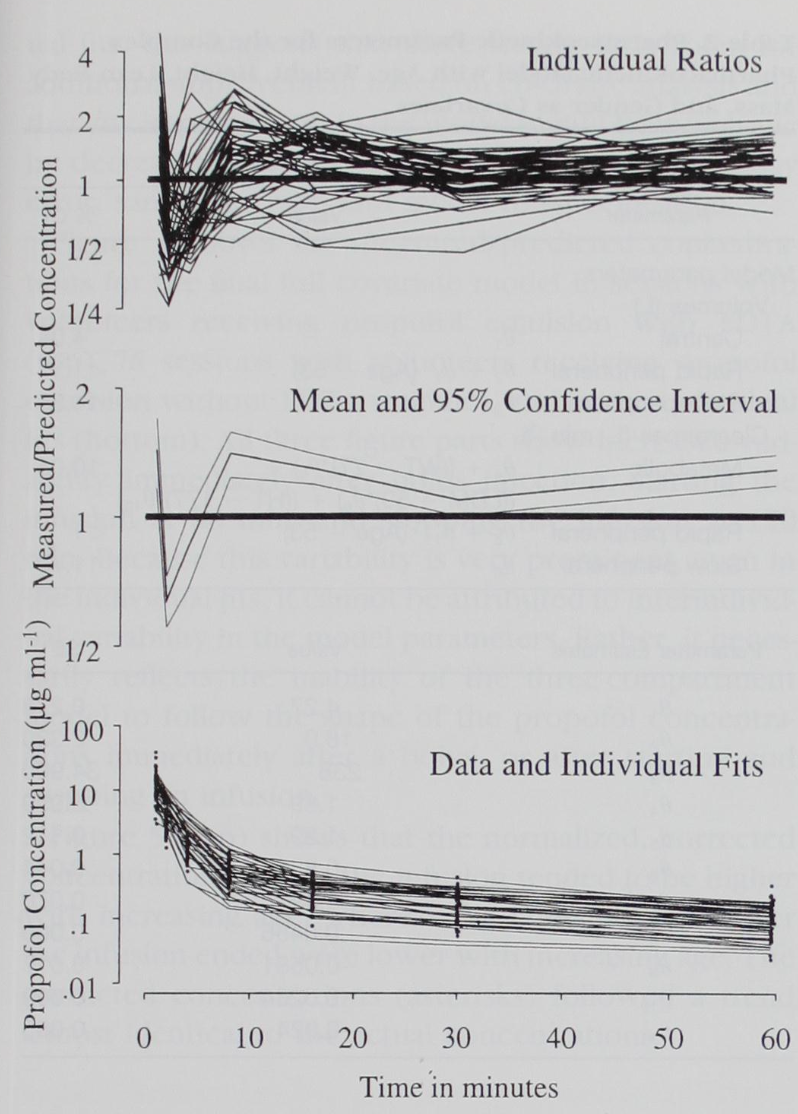
Figure 1: (Top) The ratio of each volunteer's concentrations after bolus injection to the predicted concentrations based on the infusion data from the same study session. (Middle) The mean ratio at each point in time (solid line), surrounded by 95% confidence bands (dashed lines). The bias is statistically significant, as the confidence bands consistently exclude 1. The bias is unlikely to be clinically significant, however (bottom) because the individual fits (dashed lines) describe the data (solid circles) with little visible bias.
Commentary and Notes
The negative bias at 2 and 4 minutes makes physical sense. The bolus is delivered over ~20 seconds into a forearm vein, and there is a mixing delay before it shows up in the plasma samples. The three-compartment model has no way to capture that lag, so it overpredicts concentration immediately after the bolus.
After that, the bias flips positive. The model underpredicts concentration. This supports the non-linearity hypothesis from the introduction: at bolus-level doses, the liver cannot clear propofol as fast as the linear model assumes, so it lingers longer than expected.
The key takeaway is the last sentence. The bias is statistically significant, but small relative to the inter-individual variability already present in the data. This means the infusion PK model CAN be used as a reasonable approximation for bolus dosing within the clinical range. Not perfect, but good enough to be clinically useful.
An alternative explanation involves venous-to-arterial transit time. At t=0, the bolus is injected into a forearm vein. The three-compartment model immediately assumes the drug is in plasma and begins clearing it. In reality, the drug must first travel through the venous circulation, the pulmonary circulation, and back to the arterial side before it appears at the radial artery sampling site. At t=2 and t=4 min, the model predicts high plasma concentration while the actual measured arterial concentration is still low because the drug is still in transit. This is the source of the early negative bias.
After t=4, the drug has arrived in arterial circulation and is actually peaking. But the model has been clearing drug since t=0, so it already predicts a declining concentration while the actual concentration is still rising or just peaked. From this point on the model is always behind. It consumed its predicted drug too early, so measured exceeds predicted, giving persistent positive bias. The model has no concept of the delay between venous injection and arterial appearance, and that structural gap drives the bias pattern across the entire bolus phase.
Results - Influence of Infusion Rate [Paragraph 4]
"(Figure 2) shows the concentrations observed after four different infusion rates, each demarcated by a unique line type. The concentrations are all normalized to the infusion rate, using the correction for the prior bolus dose described in methods. Figure 3suggests that the normalized, corrected concentrations are indistinguishable for the four different infusion rates."
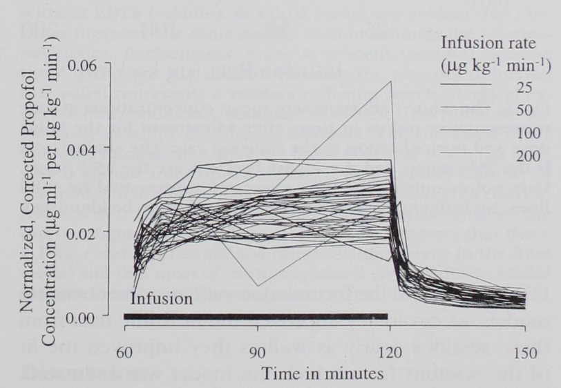
Figure 2: The concentrations observed during the infusion, adjusted for the effect of the bolus dose and normalized to the infusion rate. Each different rate is represented by a separate line type, as indicated on the legend. No evidence of nonlinearity can be identified visually.
Commentary and Notes
To reiterate, linearity would mean that double the infusion rate results in double the concentration measured in the blood. Conversely, dividing all concentrations by their respective infusion rate should results in a collection of indistinguishable lines $\pm$ some noise, as we see in Figure 2.
Results - Influence of Infusion Rate Cont. [Paragraph 5]
"(Figure 3) shows the means (white bands) and distributions for the normalized, corrected concentrations in the four infusion rate groups at four representative time points. There is no suggestion that any single group has concentrations either higher or lower than would be expected based on simple linear pharmacokinetics. Therefore, the levels in the 50-$ \mu \text{g} \cdot \text{kg}^{-1} \cdot \text{min}^{-1} $ group are nearly exactly twice the levels in the 25-$ \mu \text{g} \cdot \text{kg}^{-1} \cdot \text{min}^{-1} $ group, and the levels in the 100- and 200-$ \mu \text{g} \cdot \text{kg}^{-1} \cdot \text{min}^{-1} $ groups are the respective expected proportions higher than the 25- and 50-$ \mu \text{g} \cdot \text{kg}^{-1} \cdot \text{min}^{-1} $ groups. When the concentrations are divided by the infusion rates, the groups are indistinguishable. Therefore, the pharmacokinetics of propofol are linear from 25 to 200 $ \mu \text{g} \cdot \text{kg}^{-1} \cdot \text{min}^{-1} $. The lack of an effect of infusion rate on the concentrations was confirmed by the Kruskal-Wallis non-parametric analysis of variance, which identified no significant differences between the groups (P = 0.12)."
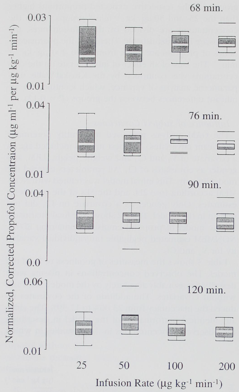
Figure 3: The white bars represent mean concentrations at four representative points in time, after adjustment for the bolus dose and normalization to the infusion rate. The shaded area is the 75% range, and the square brackets are the 95% range. Data points outside the 95% range are represented by solid lines. No influence of rate on concentration can be identified.
Commentary and Notes
Wouldn't the large effects of the covariates result in normalized concentrations that don't overlap? Well, this doesn't happen because the effects of the covariates are essentially averaged out over the population of each group. Each group had six volunteers with 2 from each age stratum (18-34, 35-65, > 65), so each group had a similar mixture of covariates. Regardless, it would be more convincing with a much larger study.
Results - Influence of Subject Covariates [Paragraph 6]
"The GAM analysis was used to identify potentially significant covariates. The best models included age as a covariate of $\text{V}_2$ and $\text{Cl}_2$ and weight, height, LBM, and gender as covariates of $\text{Cl}_1$. All parameters entered the model linearly. This initial model was refined with NONMEM according to -2LL and the SEs of the parameter estimates. Only gender as a covariate on $\text{Cl}_1$ did not remain in the model. Table 2 shows the final pharmacokinetic model of propofol emulsion containing EDTA. NONMEM estimated negligible interindividual variability for $\text{V}_2$ and $\text{Cl}_2$."
Table 2. Pharmacokinetic Parameters for the Complex Pharmacokinetics Model with Age, Weight, Height, Lean Body Mass, and Gender as Covariates| Parameter | Estimate | SE |
|---|---|---|
| $\theta_1$ | 4.27 | 0.278 |
| $\theta_2$ | 18.9 | 2.330 |
| $\theta_3$ | 238 | 34.900 |
| $\theta_4$ | 1.89 | 0.059 |
| $\theta_5$ | 1.29 | 0.112 |
| $\theta_6$ | 0.836 | 0.044 |
| $\theta_7$ | -0.391 | 0.070 |
| $\theta_8$ | 0.0456 | 0.009 |
| $\theta_9$ | -0.0681 | 0.017 |
| $\theta_{10}$ | 0.0264 | 0.009 |
| $\theta_{11}$ | -0.024 | 0.005 |
Commentary and Notes
Equation time! Recall that $\text{V}_1$ is plasma volume, $\text{Cl}_1$ is metabolic clearance (out of plasma), $\text{V}_2$ is rapid peripheral volume, $\text{Cl}_2$ is rapid peripheral clearance, $\text{V}_3$ is slow peripheral volume, and $\text{Cl}_3$ is slow peripheral clearance.
Volumes $\left[ \text{L} \right]$ $$ \begin{aligned} \text{V}_1 &= \theta_1 \\ \text{V}_2 &= \theta_2 + \theta_7 \cdot (\text{age} - 53) \\ \text{V}_3 &= \theta_3 \end{aligned} $$
Clearances $\left[ \text{L} \cdot \text{min}^{-1} \right]$ $$ \begin{aligned} \text{Cl}_1 &= \theta_4 + \theta_8 \cdot (\text{wt} - 77) + \theta_9 \cdot (\text{lbm} - 59) + \theta_{10} \cdot (\text{ht} - 177) \\ \text{Cl}_2 &= \theta_5 + \theta_{11} \cdot (\text{age} - 53) \\ \text{Cl}_3 &= \theta_6 \end{aligned} $$
Coefficients of Variation $$ \begin{aligned} \text{V}_1 & \quad : \quad 4.04 \\ \text{V}_2 & \quad : \quad \lt 1 \\ \text{V}_3 & \quad : \quad 14.35 \\ \text{Cl}_1 & \quad : \quad 10.05 \\ \text{Cl}_2 & \quad : \quad \lt 1 \\ \text{Cl}_3 & \quad : \quad 11.79 \end{aligned} $$
Gender dropped out of the final model despite being flagged by GAM. GAM finds candidates, but NONMEM is confirmatory and applies a stricter ±2 SE test, which Gender didn't survive.
Negligible inter-individual variability on $\text{V}_2$ and $\text{Cl}_2$ means age explains those parameters well.
All covariates exist as linear relationships in the formulas. GAM could have found nonlinear relationships but didn't, which keeps the model simple and interpretable. This also allows for a lot of convenient mathematical shortcuts via closed-form solutions, but we will get there in subsequent writeups.
To generate a virtual patient given demographics $\{\text{age}, \text{ht}, \text{wt}, \text{lbm}\}$, first compute the typical value from the covariate equations, then apply a log-normal perturbation using the CV: $$P_i = P_{\text{TV}}(\text{covariates}) \cdot e^{\eta_i}, \quad \eta_i \sim \mathcal{N}(0,\, \omega^2)$$ where $\omega \approx \text{CV}/100$ for small CV. For example, to generate $\text{V}_{1,i}$ for a virtual patient: $$\text{V}_{1,i} = \theta_1 \cdot e^{\eta_i}$$ and to generate $\text{Cl}_{1,i}$: $$\text{Cl}_{1,i} = \left[\theta_4 + \theta_8 \cdot (\text{wt} - 77) + \theta_9 \cdot (\text{lbm} - 59) + \theta_{10} \cdot (\text{ht} - 177)\right] \cdot e^{\eta_i}$$ Each parameter gets its own independently sampled $\eta_i$ with its own $\omega$ from the CV column of Table 2. Parameters with negligible CV ($\text{V}_2$, $\text{Cl}_2$) are treated as fixed at their typical values, so no random perturbation is needed.
Results - Influence of Subject Covariates Cont. [Paragraph 7]
"Table 3 shows the measures of goodness of fit of the model. The observed concentrations in plasma were described reasonably accurately by the models with and without covariates. The addition of the covariates reduced the inaccuracy from 23.00% to 17.39%. The virtually identical performance of the model in describing the observed concentrations in those studies in which EDTA was not in the formulation validated the covariate models, as covariates improved the fit to the data from these sessions nearly as well as they improved the fit of the sessions from which the model was estimated. The individual fits show a MDAWR of 14.18%, which was very nearly the residual error seen in the full covariate model. As the covariates could not possibly do any better than the model parameters estimated in individual fits, this suggests that there is very little room for additional improvement based on covariate analysis and that any improvement in the model would have to come by decreasing sources of intrasubject variability: assay error, sampling error, and model misspecification."
Table 3. The population model with and without covariates was estimated from observed concentrations following administration of propofol with EDTA. Weighted residuals are in-sample (the data the model was estimated from). Performance error is out-of-sample (propofol without EDTA), serving as a validation set. Individual fits were performed per study session, so no performance error column applies.
Table 3. Measures of Goodness of Fit| Model | Weighted Residuals (%) | Performance Error (%) |
|---|---|---|
| No covariates | ||
| Median | -1.56 | -3.16 |
| Median absolute | 23.00 | 21.56 |
| Covariate | ||
| Median | -1.86 | -2.98 |
| Median absolute | 17.39 | 18.63 |
| Individual fits | ||
| Median | 0.31 | |
| Median absolute | 14.18 |
Commentary and Notes
MDAWR collapses all observations from all patients into a single number, so it is dominated by intrasubject noise: assay error, sample timing error, and the fact that a 3-compartment model is a simplification of reality. Covariates do not fix that noise. They fix which curve each patient sits on, shifting the predicted trajectory to match that patient's physiology.
The individual fits floor (14.18%) is the key reference point. It was calculated by fitting a separate set of PK parameters to each patient's actual measured concentration-time data, with no demographic constraints. This is purely retrospective and cannot be used clinically since you need the full measurement history to compute it. That makes it the theoretical best this 3-compartment population model could ever do: a population model has to predict parameters before seeing any measurements, using only demographics. The gap between no covariates (23.00%) and individual fits (14.18%) is about 9 percentage points, which is the total explainable inter-patient variance. The covariate model (17.39%) recovers most of that gap, leaving only about 3 points on the table.
So covariates are not doing little. They are recovering most of what is recoverable. The remaining 14% is irreducible intrasubject noise.
Results - Influence of Subject Covariates Cont. [Paragraph 8]
"Figure 4 shows the measured/predicted concentrations for the final full covariate model in sessions with volunteers receiving propofol emulsion with EDTA (top), in sessions with volunteers receiving propofol emulsion without EDTA (middle), and in the individual fits (bottom). All three figure parts show increased variability immediately after bolus injection, starting the infusion at 60 min, and stopping the infusion at 120 min. Because this variability is very prominent, even in the individual fits, it cannot be attributed to interindividual variability in the model parameters. Rather, it necessarily reflects the inability of the three-compartment model to follow the shape of the propofol concentrations immediately after a bolus, or after starting and stopping an infusion."
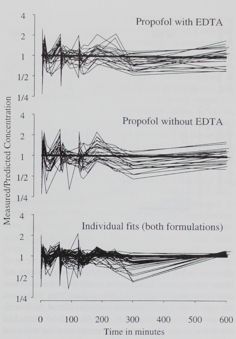
Figure 4: The ability of the final pharmacokinetic model, including covariates, to describe the concentrations observed after administration of propofol emulsion with EDTA (top) and without EDTA (middle). Residual errors are evident (top) because these are the same studies used to estimate the pharmacokinetics. Performance error is evident (middle) because these data were not used to estimate the pharmacokinetics; this panel represents a validation during nearly identical experimental conditions. Residual errors from individual fits for all study sessions are shown (bottom). The increased error (bottom) immediately after the bolus dose and when the infusion is started and stopped reflects a fundamental inability of the model to accommodate the shape of the observed concentrations over time. The similarity in overall error between the top two figure parts and the bottom part suggests that there is little residual unexplained interindividual error in the final model and that most of the unexplained error is due to model misspecification and measurement error.
Commentary and Notes
This paragraph is the visual confirmation of what Table 3 showed numerically. The spikes in the measured/predicted ratio appear at three moments: the bolus at t=0, infusion start at t=60, and infusion stop at t=120. Critically, those spikes are visible in all three panels, including the individual fits at the bottom.
That matters because individual fits use patient-specific parameters. If the spikes were caused by using the wrong parameters for a patient, they would disappear in individual fits. They do not. The only remaining explanation is that the 3-compartment model is structurally unable to track the shape of concentrations during rapid transitions. This is model misspecification, and it is part of what sets the 14.18% individual fits floor.
The EDTA validation is also visible here. The top and middle panels (with and without EDTA) look nearly identical in spread, which is consistent with the PE numbers in Table 3 tracking closely with the WR numbers across both models.
Results - Influence of Subject Covariates Cont. [Paragraph 9]
"Figure 5 (top) shows that the normalized, corrected concentrations during the infusion tended to be higher with increasing age, whereas the concentrations after the infusion ended were lower with increasing age. The predicted concentrations (asterisks) followed a trend almost identical to the actual concentrations."
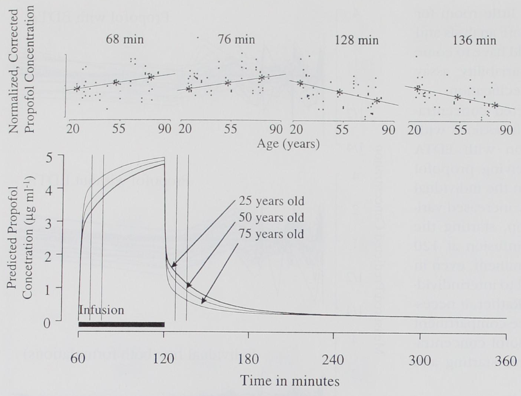
Figure 5: Comparison of the measured with the predicted concentrations during the infusion. The four graphs show the relationship of the normalized, corrected concentrations at 68, 76, 128, and 136 min to age. The line through the data is a linear least-squares fit. The asterisks represent the predicted normalized concentration for a 77-kg, 175-cm woman at ages 25, 50, and 75 yr. During the infusion, concentrations tended to be higher in the elderly, whereas after the end of the infusion the opposite was observed. The full time course of the predicted concentrations after an infusion at 200 $\mu\text{g} \cdot \text{kg}^{-1} \cdot \text{min}^{-1}$ is shown (bottom). The vertical lines represent the four time points chosen for the comparison above.
Commentary and Notes
This figure is the visual proof that the age covariate in the model captures something real. Older patients accumulate more drug during infusion (higher normalized concentrations at t=68 and t=76) but clear it faster after the infusion stops (lower normalized concentrations at t=128 and t=136).
The mechanism is in the covariate equations. Age appears in both $V_2$ and $\text{Cl}_2$, meaning older patients have a smaller rapidly equilibrating compartment and slower inter-compartmental clearance. During infusion, drug accumulates in plasma more because it distributes less readily into $V_2$. After infusion stops, there is less drug stored in $V_2$ to return to plasma, so concentrations fall faster.
The asterisks (model predictions at ages 25, 50, 75) track the measured trend closely, which validates that the model is capturing the age effect correctly rather than just fitting noise.
Results - Influence of Disodium Edetate on Pharmacokinetics of Propofol [Paragraph 10]
"Figure 6 shows the ratio of concentrations after administration of propofol emulsion without EDTA to administration of propofol emulsion with EDTA in each individual over time. There is no suggestion in Figure 6that the presence of EDTA resulted in any systematic difference in concentration between the two groups. Figure 6 (bottom) shows the mean and 95% confidence interval over time. The mean ratios ranged from 0.96 to 1.15. The bounds included 1 at each time, strongly suggesting that the concentrations in plasma after administration of propofol emulsion are not influenced by the presence of EDTA in the formulation. The results of this nonparametric method are consistent with the validation of the pharmacokinetic model mentioned previously: The model derived from the formulation containing EDTA performed just as well describing the data from the formulation without EDTA as it did describing the data from which it was derived."
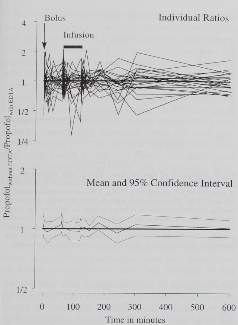
Figure 6: The ratio of concentrations after administration of propofol without EDTA to administration with EDTA at each time point for each volunteer is shown (top). The mean ratio (solid line) and 95% confidence bounds (dashed lines) are shown (bottom). The confidence bounds include 1 at each time point, confirming that the pharmacokinetics of propofol are not influenced by EDTA.
Commentary and Notes
This paragraph ties the EDTA question together with two independent lines of evidence pointing to the same conclusion. First, the nonparametric comparison: each volunteer's ratio of without-EDTA to with-EDTA concentration is plotted over time. If EDTA systematically altered PK, you would expect the ratios to drift away from 1 in a consistent direction. They do not. The 95% CI on the mean ratio contains 1 at every time point, with the mean ranging only from 0.96 to 1.15.
Second, the model validation: the covariate model estimated on the with-EDTA data described the without-EDTA data just as well (PE tracked WR in Table 3). If EDTA changed the underlying PK, that cross-prediction would have failed. It did not.
Two methods, one conclusion: EDTA has no meaningful effect on propofol pharmacokinetics.
Discussion
For the discussion section, I'm going to leave the authors more room to explain their reasoning before adding my own commentary.Discussion - Influence of Method of Administration [Full]
"In this study, the pharmacokinetics based on the infusion data generally underpredicted the observations after the bolus dose. The main difference between the bolus and infusion data was the much higher concentration immediately after the bolus dose. Not only was the high 1-min concentration underpredicted, however, but also the lower values 8, 15, 30, and 60 min after the bolus dose. These measurements were in the concentration range observed during and after the infusion."
"Studies with computer-controlled infusion pumps have provided additional evidence that the mode of drug administration influences the pharmacokinetics of propofol. In these studies, pharmacokinetic models derived from studies with a bolus dose and a brief infusion [6,9,22,23] have predicted the concentrations during the computer-controlled infusion only poorly. It is noteworthy that parameters from a bolus dose-only study with propofol [2] resulted in the worst prediction of five evaluated parameter sets. [6]"
"One possible explanation for this persistent difference could be physiologic. Lange et al. [24] observed that after a 2.0-mg/kg bolus dose of propofol for induction of anesthesia for cardiac surgery, blood flow in the liver was reduced by 14%. This reduction continued until sternotomy. Therefore, it appears from these data and the results of the current study that bolus doses of propofol cause a small but persistent change in blood flow in the liver, resulting in decreased clearance and concentrations higher than those predicted from infusion data. This mechanism could explain the underprediction of most of our postbolus concentrations, especially if the change in blood flow in the liver is long-lasting, but does not explain the overprediction of the 2- and 4-min values."
"Another possible explanation is model misspecification. Pharmacokinetic models typically assume that the central compartment is well stirred. That is, an injected bolus dose of propofol is assumed to distribute immediately and homogeneously in the central compartment. Investigations by Henthorn et al. [25] and Krejcie et al., [26] however, have demonstrated multiple peaks after bolus injection because of rapid recirculation. Because traditional compartmental models are represented by monotonic functions, these recirculation oscillations cannot be described. Therefore, no conventional compartmental model can properly describe the actual concentrations after bolus injection. The inability of our three-compartment model to describe the initial high peak is certainly consistent with this type of model misspecification, but the influence of recirculation on some of the later postbolus values should be negligible. Further, it should be kept in mind that all models are, by definition, simplifications of complex physiologic processes that may change with time and drug concentration. In all likelihood, both decreased blood flow in the liver and model misspecification played a part in the suboptimal prediction of the postbolus concentrations by the models derived from infusion data only."
Commentary and Notes
The authors propose three mechanisms to explain why the infusion model mispredicts bolus concentrations.
For the early overprediction at t=2 and t=4 min, they point to the well-stirred assumption. A compartmental model assumes a bolus instantaneously distributes homogeneously in plasma. In reality, bolus injection produces recirculation oscillations, meaning concentration peaks multiple times as the drug loops through the cardiovascular system. A 3-compartment model is a monotonically declining function after the initial peak, so it structurally cannot represent those oscillations. Our earlier commentary attributed this early bias to venous-to-arterial transit time, which is a related but distinct framing: the drug has not yet arrived at the arterial sampling site while the model has already assumed it is in plasma and clearing. Both explanations point to the same root cause: the model assumes instantaneous mixing that does not happen.
For the persistent underprediction after t=4 min, the authors cite Lange et al., who measured a 14% reduction in hepatic blood flow following a propofol bolus. Since propofol clearance is flow-dependent, reduced hepatic blood flow means reduced clearance, so drug lingers longer than the model predicts. This is a physiologic mechanism, not a modeling assumption, and it only applies at bolus-level doses where the transient hemodynamic effect is large enough to matter.
The authors conclude both mechanisms likely contributed. Neither alone fully explains the bias pattern, and they are not mutually exclusive.
A third mechanism is worth considering. Because the 3-compartment model is integrated forward in time, each state depends on the previous: $$x(t + dt) = x(t) + \frac{dx}{dt} \cdot dt$$ The well-stirred assumption means the model starts clearing drug from t=0, while in reality the drug has not yet arrived at the arterial sampling site. By the time the drug arrives, the model has already eliminated a fraction of the dose equal to $1 - e^{-k_e \cdot \tau}$, where $\tau$ is the transit delay. From that point on, the true and model systems decay at the same rate, so the ratio of true to predicted concentration locks in as a fixed constant and never converges back to 1.
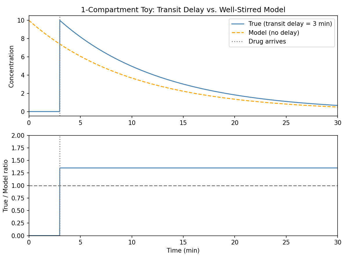
Toy 1-compartment simulation with a 3-minute transit delay. The model (no delay) starts clearing immediately, so when the drug arrives the model is already behind. The ratio locks in at ~1.35 and stays flat indefinitely, demonstrating that transit delay alone can produce persistent bias with no change in clearance parameters.
This is mathematically distinct from the hepatic blood flow explanation. Reduced hepatic clearance changes $k_e$, causing the two curves to diverge over time. Transit delay produces a fixed multiplicative offset from the moment drug arrives, with both curves decaying at the same rate. The flat ratio in the toy example is the signature of this mechanism. Whether it is the dominant effect in the real data is unknown, but it is physically plausible, mathematically possible, and requires no change in underlying physiology or a non-linear, more complicated model.
Discussion - Influence of Infusion Rate [Full]
"Linearity can be understood in terms of the superposition principle, which says that the concentration obtained from multiple simultaneous infusions is the same as the sum of the concentrations when the infusions are given separately. This is only the case if no saturation effects are evident. That is, doubling the infusion rate doubles the concentrations. If a clearance saturates at a particular infusion rate, then increasing the rate results in a greater than proportional increase in concentration."
"Evidence for nonlinearity was discussed recently by Coetzee et al. [9] A parameter set obtained from a majority of blood samples with subanesthetic concentrations consistently underpredicted the concentrations during the computer-controlled infusion. Vuyk et al. [6] also observed an underprediction of high concentrations in plasma with these parameters. They conjectured that the nonlinearity of the kinetics of propofol might explain the findings. An investigation of Bailey et al. [7] in patients undergoing coronary revascularization, however, found no evidence for nonlinearity. A linear relationship between concentration at steady state and infusion rate also was found in patients during regional anesthesia. [1]"
"In the current study, the normalized, corrected concentration measurements during the infusion were independent of the rate. This is graphically expressed in Figure 2 and Figure 3. There was no evidence for nonlinearity over the range of infusion rates studied. A possible source of bias in our analysis, however, could have come from the subtraction of predicted bolus values from the measured concentrations. Although both bolus and infusion data were used in this set of analyses and the bolus phase was probably represented more accurately, if the bolus concentrations were underpredicted, as in the analysis here, this would make the adjusted concentrations proportionately higher in the lower infusion rate groups, thereby masking the nonlinearity as reported by Coetzee et al. [9] and Vuyk et al. [6]"
"A recent study may shed light on the apparent discrepancy among studies that demonstrate linearity and those that do not. Pavlin et al. [27] observed a pharmacokinetic interaction of propofol and alfentanil in a well-controlled volunteer study. The concentrations of propofol were considerably higher when alfentanil was infused concurrently with alfentanil compared with an infusion of the propofol alone. Altered first-pass uptake of propofol in the lung [28,29] or changes in blood flow in the liver might have been causal for this pharmacokinetic interaction. It is possible that the nonlinearity in the pharmacokinetics of propofol discussed by Coetzee et al. [9] and Vuyk et al. [6] may have been due to a pharmacokinetic interaction between propofol and opioids."
Commentary and Notes
Linearity here means superposition: double the infusion rate, double the steady-state concentration. It holds as long as clearance is not saturated. This paper found no evidence of nonlinearity between 25 to 200 $\mu\text{g} \cdot \text{kg}^{-1} \cdot \text{min}^{-1}$ in volunteers receiving propofol alone.
The conflict with Coetzee and Vuyk (who did find apparent nonlinearity) is left open with two hypotheses. First, the authors acknowledge a potential bias in their own analysis: since bolus concentrations were underpredicted, subtracting those underpredicted values from measured concentrations would inflate the adjusted values more in lower infusion rate groups, which could mask nonlinearity. So their linearity finding is not airtight.
Second, Pavlin et al. suggest the apparent nonlinearity in those earlier studies may not have been dose-dependent at all. Propofol combined with opioids produces higher propofol concentrations than propofol alone, possibly due to altered first-pass lung uptake or changes in hepatic blood flow. If those earlier studies used opioids concurrently, the apparent nonlinearity could have been a drug-drug interaction rather than clearance saturation.
Whether propofol PK is truly linear in the presence of opioids is a question this paper cannot answer. Later papers will confirm or deny these hypotheses in more clinical settings.
Discussion - Influence of Subject Covariates [Full]
"Covariate models attempt to explain and thereby reduce the interindividual variability of the parameters. We derived a full pharmacokinetic model using the data from the administration of propofol with EDTA, using a GAM analysis to identify potentially significant covariates. All the covariates detected by the GAM analysis were tested for significance using the objective criterion of NONMEM. After deleting gender, the remaining covariates were significant based on the -2LL and the SE. Age was significant for $\text{V}_2$ and $\text{Cl}_2$. This indicates that intercompartmental drug distribution is influenced by age. The metabolic clearance is influenced by weight, LBM, and height. Although weight, LBM, and height all correlate with each other, inclusion of all three covariates improved the fit significantly ($\text{P} \lt 0.01$) compared with inclusion of any combination of just two of these covariates. Most previously published pharmacokinetic models for propofol have been weight proportional. [4,5,21] Only Dyck et al. al.* and Kirkpatrick et al. [2] found an effect of age. The effect of age we found for propofol in our study looks similar to that found for thiopental in other studies. [30,31]"
"The age stratification of our study population made these data well suited to detection of an effect of age, although the lower bolus dose received by the volunteers older than 65 yr may have been a confounding factor. We addressed the latter issue by comparing the model prediction with the normalized, corrected concentrations. During the infusion, the normalized, corrected concentrations are higher in the elderly, whereas the concentrations are lower after the infusion is stopped. The model also predicts age-related changes of very similar magnitude. Although we cannot be sure that we are subtracting the correct bolus contribution to obtain the normalized, corrected concentrations, it is probable that age is an important independent covariate. To illustrate the influence of age on dose, we calculated the infusion rates required to reach and maintain a concentration of propofol in plasma of 3.5 $\mu \text{g} \cdot \text{ml}^{-1} $ micro gram/ml with a computer-controlled infusion pump in the same hypothetical volunteer as before at ages 25, 50, and 75 yr. The time course of the infusion rates shows that younger people need higher infusion rates during the first 20-30 min to achieve the same concentration (Figure 7). A noteworthy corollary from the data and the simulations is that older people have a faster decrease in concentration after an infusion is stopped."
"The covariate-adjusted pharmacokinetic model for propofol with EDTA accurately described the concentrations observed after administration of the propofol without EDTA. Figure 5(top and middle) shows that the residual error and the prospectively applied performance error were of similar magnitude. The best possible description of pharmacokinetic data with a three-compartment model was obtained with individual fits (Figure 5, bottom). The remaining inaccuracy is mostly due to measurement error or model misspecification. Because the accuracy of the covariate-adjusted model closely approaches that of the individual fits, further refinements in the pharmacokinetics of propofol cannot be expected from further inclusion of covariates."
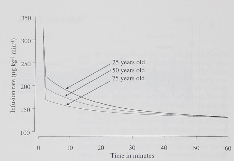
Figure 7: Influence of age on dose. The y axis represents the computer-controlled infusion rates for a target concentration of 3.5 $\mu\text{g} \cdot \text{ml}^{-1}$ in a 77-kg, 175-cm woman at ages 25, 50, and 75 yr. In younger people, higher infusion rates must be maintained during the first 20-30 min. In elderly people, after the first minute, a constant infusion rate is adequate to maintain a constant plasma concentration.
Commentary and Notes
This section is the authors closing the loop on the covariate model. The two-stage process (GAM to find candidates, NONMEM to confirm) was covered in the Methods section. Here they explain what the surviving covariates mean physiologically.
Age affecting $\text{V}_2$ and $\text{Cl}_2$ means aging changes how quickly drug distributes into and returns from the rapidly equilibrating compartment. The consequence is visible in Figure 7: younger patients need higher infusion rates for the first 20-30 min because drug is rapidly leaving the plasma into $\text{V}_2$. Older patients have slower inter-compartmental exchange, so plasma concentration builds up more readily and a lower, flatter infusion rate suffices. The flip side is that older patients also see a faster concentration drop after infusion stops, since there is less drug stored in $\text{V}_2$ to return to plasma.
The note that weight, LBM, and height all correlate with each other yet all three independently improved the fit is worth flagging. This is a multicollinearity situation: including correlated predictors can inflate standard errors and make individual coefficients unstable. The authors justify inclusion by the significant -2LL improvement, but it also means the individual coefficients for weight, LBM, and height should be interpreted with caution rather than in isolation.
The final paragraph re-states the conclusion from Table 3: the covariate model nearly matches the individual fits floor, so additional covariates are unlikely to help. Any remaining error is intrasubject noise and model misspecification, not unexplained interindividual variability.
Discussion - Influence of Disodium Edetate on Pharmacokinetics of Propofol [Full]
"The small quantity of EDTA added to propofol ($lt$ 1%) was not expected to alter the pharmacokinetic profile remarkably. The toxicity of EDTA when infused at high rates has been investigated and reported by Dudley et al. [32] in 1955 and by Meltzer and colleagues in 1961. [33] In most patients, they observed moderate orthostatic hypotension. As hypotension can be associated with reduced blood flow in the liver, this suggests the possibility that EDTA might reduce clearance of propofol. Bolus injections of propofol without EDTA have been shown to reduce blood flow in the liver. [24] It was theoretically possible that the addition of EDTA to the formulation of propofol might exacerbate the hypotensive effects of a bolus dose, further reducing blood flow in the liver and altering clearance of propofol."
"The crossover study design allowed for direct comparison of the concentration values between formulations with and without EDTA under otherwise identical experimental conditions. This approach eliminated the possible influence of model misspecification on the result. Multiple comparisons with t tests normally require correction of the significance level. We were not concerned about falsely rejecting the null hypothesis (the ratio of the concentrations equals 1). Therefore, our decision to not correct the level of significance represented a conservative approach. Using this approach, a mean ratio of $\gt$ 1.17 or $\lt$ 0.83 at any time point could have been detected with 80% power; our mean ratios were always within this range. Our conclusion, therefore, was that EDTA did not alter the pharmacokinetics of propofol."
Commentary and Notes
The first paragraph lays out the theoretical concern: EDTA at high infusion rates causes hypotension, hypotension reduces hepatic blood flow, and propofol clearance is flow-dependent. So there was a plausible mechanism by which EDTA could reduce clearance and inflate propofol concentrations.
The second paragraph explains the statistical framing, which connects directly to our earlier commentary on Bonferroni correction. The null hypothesis is that the concentration ratio equals 1. They were not worried about falsely rejecting the null (a Type I error), meaning they were not worried about concluding EDTA has an effect when it does not. They were worried about the opposite: failing to detect an effect that is actually there (Type II error). By not applying a multiple comparisons correction, they kept the confidence interval narrow, making it harder for the mean ratio to stay within bounds at every time point. The fact that it did (with mean ratios always between 0.83 and 1.17) makes the no-effect conclusion more credible.
The 80% power statement tells you the minimum detectable effect size: a ratio outside [0.83, 1.17] at any time point would have been detected with 80% probability. Their observed ratios were 0.96 to 1.15, sitting comfortably inside that window. EDTA, at the concentration added to propofol, does not meaningfully affect its pharmacokinetics.
Conclusion
"The addition of EDTA does not alter the pharmacokinetics of propofol. An induction bolus dose has a different kinetic profile than infusion rates between 25 and 200 $\mu \text{g} \cdot \text{kg}^{-1} \cdot \text{min}^{-1} $. The difference is statistically significant, but its effect in predicting a measured concentration is small compared with the overall pharmacokinetic variability of propofol among different patients. The pharmacokinetics of propofol are linear for clinically relevant infusion rates. Age, weight, height, and LBM are significant covariates for propofol pharmacokinetics. “Prospective” evaluation of the derived parameters during nearly identical experimental conditions with the same volunteers showed performance errors that were of the same order of magnitude as the WRs in the model from which the parameters were derived."
"The authors thank Carol A. Cohane, R.N., Kimberly J. Stoughton, and Lola Bozovich for their assistance in all phases of the study; Keith Gregg for statistical assistance; and Deborah Raybuck and Virginia Crego for performance of the propofol assay."
My Key Takeaways
- EDTA does not affect propofol pharmacokinetics. Despite a plausible physiologic mechanism (EDTA causes hypotension, hypotension reduces hepatic blood flow, propofol clearance is flow-dependent), the crossover study found mean concentration ratios always within 0.96 to 1.15. Both the nonparametric ratio analysis and the model's equal performance on EDTA-free data point to the same conclusion.
- Bolus dosing produces a different kinetic profile than infusion. The 3-compartment model estimated from infusion data systematically mispredicts post-bolus concentrations: it overpredicts at t=2,4 min and underpredicts persistently after that. The bias is statistically significant but small relative to overall inter-patient variability, meaning the infusion model is still a reasonable clinical approximation for bolus dosing. Two mechanisms likely contribute: recirculation oscillations the model cannot represent (well-stirred assumption), and reduced hepatic blood flow at bolus-level doses. A third mechanism is also plausible: the transit delay from venous injection to arterial sampling puts the model on a permanently offset trajectory from the moment the drug arrives.
- Propofol pharmacokinetics are linear over clinically relevant infusion rates (25 to 200 $\mu\text{g} \cdot \text{kg}^{-1} \cdot \text{min}^{-1}$). Apparent nonlinearity reported in earlier studies may have been a drug-drug interaction with opioids rather than clearance saturation.
- Age, weight, height, and LBM are significant covariates. Age affects $\text{V}_2$ and $\text{Cl}_2$, meaning older patients distribute drug more slowly and see faster concentration drops after infusion stops. Metabolic clearance is jointly influenced by weight, LBM, and height. Gender was flagged by GAM but did not survive the NONMEM confirmation step.
- The covariate model nearly reaches the individual fits floor. MDAWR drops from 23% (no covariates) to 17.4% (covariate model), approaching the 14.2% achievable with patient-specific parameters. The remaining error is intrasubject noise and structural model misspecification, and no additional covariates are likely to improve it further.
References
- Schnider TW, Minto CF, Gambus PL, Andresen C, Goodale DB, Shafer SL, Youngs EJ. The influence of method of administration and covariates on the pharmacokinetics of propofol in adult volunteers. Anesthesiology. 1998 May;88(5):1170-82. Full text. PMID: 9605675.
- Hepatic Extraction Ratio - ScienceDirect Topics
- Muller AE, Huisman I, Roos PJ, Rietveld AP, Klein J, Harbers JB, Dorresteijn JJ, van Steenbergen JE, Vos MC. Outbreak of severe sepsis due to contaminated propofol: lessons to learn. J Hosp Infect. 2010 Nov;76(3):225-30. doi: 10.1016/j.jhin.2010.06.003. PMID: 20692067.
Propofol is an emulsion containing soybean oil and egg lecithin (a fatty substance derived from egg yolks), making it a prime environment for bacteria to thrive. That is why the preservative EDTA (disodium edetate) was initially introduced and is still to this day (2026). Although it helps, bacterial growth from mishandling propofol is still a possibility, and it can even lead to sepsis[3]! Intravenously infusing bacteria throughout the body... not a good situation.
The paper also serves to figure out if propofol pharmacokinetics are linear, or at least linear in some region-of-interest. Additionally, they are concerned with investigating various covariates (age, weight, height, lean body mass, gender) of propofol pharmacokinetics.